Why Bayesian Probability Feels So Confusing — And Why It Doesn’t Have To Be

Note: this post is part of a Series of post about Bayesian Statistics

Hey everyone! When learning Bayesian Statistics, the very first formula you will see is Bayes Rule which looks something like that:

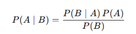
Now, if you are like me, this formula would make sense to you, yet you have this nagging feeling that you don’t fully appreciate its nuances. The reason behind it is because if you picked up statistics via the frequentist approach, you probably can’t quite grasp the idea of “conditional probability” that well. In most of our traditional frequentist statistics, we just work towards “disproving independence”.

Consider regression, where we test if the coefficient is significantly different from 0. Or a chi-square test of independence, where we reject the null hypothesis and say that the variables are not independent. Frequentist statistics stops here — we don’t deal with raw probability, or how a probability changes now that we know some information. Which is why conditional probability feels so foreign to us!

The link lies in the Chi-Square Test of Independence. Let’s examine a familiar scenario whereby we see if gender and smoking status are related. The 2x2 cross tab looks like that:

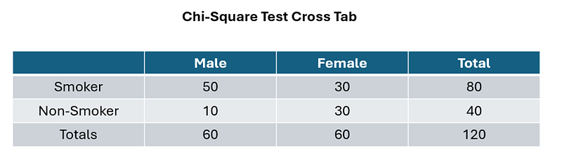
From the frequentist viewpoint, we are typically interested in testing whether gender is related to smoking status. To test this hypothesis, the procedure is simple. Simply conduct a chi-square test of independence, and you will find that the Chi-Square Test Statistic is 15, with df = 1, and p-value = 0.00010751 (I used https://www.quantpsy.org/chisq/chisq.htm to compute this easily).

Okay! So the p value is <0.05, the effect is statistically significant, and we now know that Gender is related to Smoking Status. With this result, you can go ahead and publish your research paper already — this is where the frequentist perspective typically ends.

From Frequentist to Bayesian

The Bayesian Perspective takes it a little further however — it works directly with probabilities. Via the frequentist approach, we only implicitly compute probabilities — it is possible to conduct your entire analysis without ever directly dealing with the probability directly.

Intuitively, when we say that “gender is related to smoking status”, a frequentist understands it to mean that being male/female affects the chances of you being a smoker — meaning to say that your gender provides information about whether or not you are a smoker. Drawing out a tree diagram for these probabilities, the probability if gender was related to smoking would be as follows:

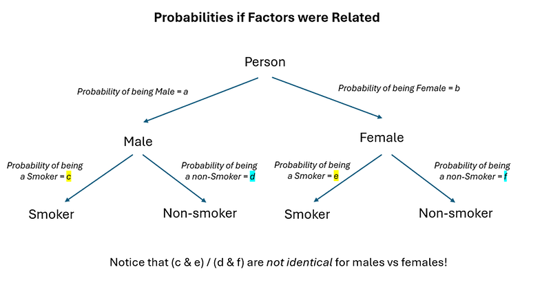
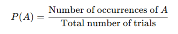
The probabilities — a,b,c & d — are relatively easy to compute. From a frequentist perspective, probability is simply:

Thus, the probability of being male is 60/120 = 50%, the probability of being female is 60/120 which is also 50%. For males, the probability of him being a smoker is 50/60 = 83.3%, whereas for females, the probability of her being a smoker is 30/60 = 50%. Let’s go ahead and fill these values inside our tree diagram.

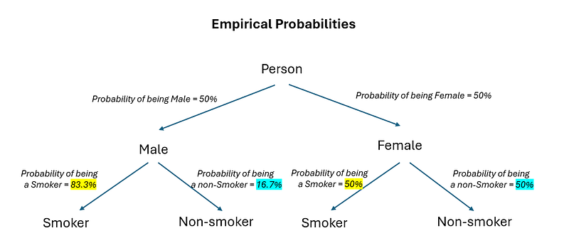
When a frequentist says that “gender is related to smoking status”, we implicitly understand that the probability of being a smoker is different for males vs females. By doing a chi-square test — what we are actually doing is testing if the difference in probability for males vs females (yellow in male vs yellow in female & blue in male vs blue in female) is large enough to constitute evidence against the null hypothesis (independence) — in which the probabilities look like this:

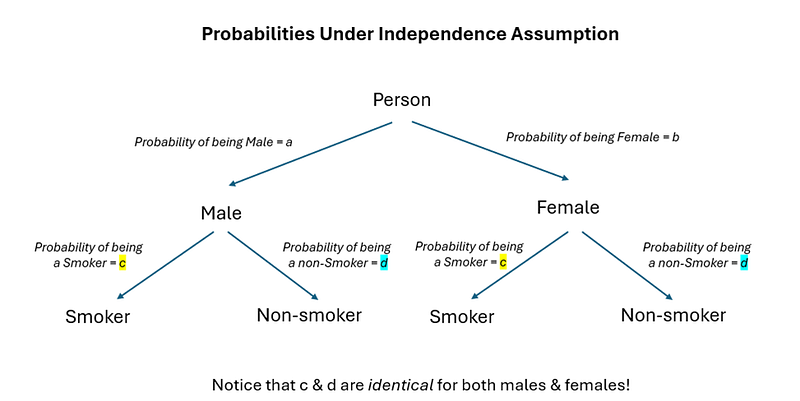
Independence implies that knowing a person’s gender does NOT change the probability of the person being a smoker — meaning that the probability of being a smoker (c & d), whether you are male or female, is identical. c & d under independence again is relatively easy to compute — it is simply the probability of a random person being a smoker, ignoring their gender (since gender is assumed to be unrelated!) As such, we can compute the probability of a random person being a smoker to be 80/120 = 66.66% (assuming the sample is representative of the population). Filling this up into our tree diagram, the probabilities under independence are as follows:

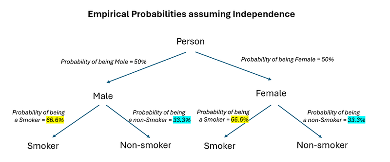
Side note: this is a good time to note that independence does NOT mean the probability of being a smoker vs non-smoker must be 50/50 for both males and females! It just means that the probability of being a smoker vs non-smoker must be equal for both males and females — which means that a 66.6/33.3 split like in the above scenario — as long as the distribution is identical for BOTH males and females — means that gender is unrelated to smoking status!

Conditional Probabilities Under Dependence vs Independence

Congrats! If you can follow what I told you, you basically have everything you need to understand Bayesian Probability. But before we go there, we have to first get one of the biggest misconceptions (and hurdles) out of the way — the computation of conditional probability.

With a tree diagram — it is very easy to compute probabilities. Just multiply the probabilities all the way to the bottom of the tree, and you will get the value you need. For instance, say you are interested in the probability of a person being a male smoker. The path you should follow is below:

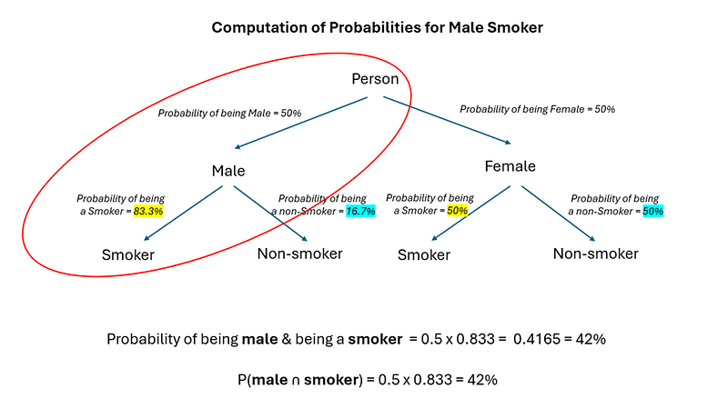
And this gives you a probability of 42%.

Based on the above, some people might conclude this:

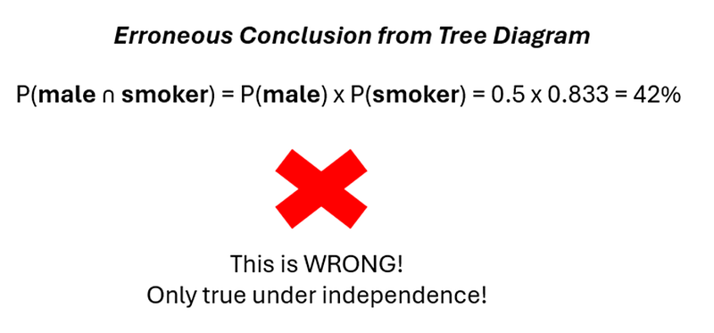
But this is WRONG. Why? Because they have forgotten that the 0.833 in the above scenario is contingent on the person ALREADY BEING MALE! The 0.833 above is a conditional probability — denoted as follows:

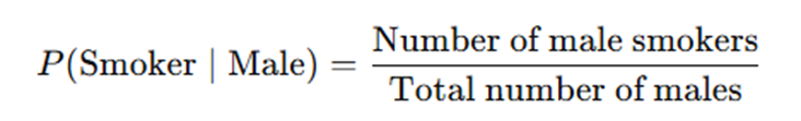
Notice that the denominator only takes into account males in the first place? This 0.833 is computed via the male subset of the entire sample already — and was obtained via 50/60! If you were to compute the probability of a person being a smoker, it would instead be this:

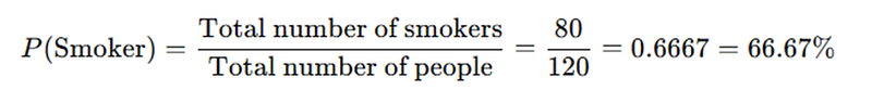
66.6% is NOT the same as 83.3%!

Default of Frequentists: Independence

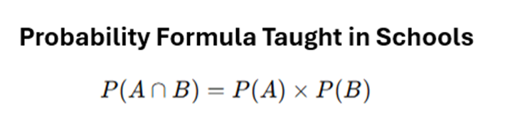
If you were like me, most of your education you are used to seeing this formula:

Based on the above probabilities, I can already see you rushing out the computation in your head:

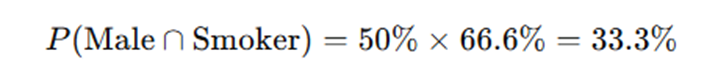
But this is not the same probability as we previously computed from our tree diagram (42%) — why?

Because the Probability Formula you learnt was wrong!

P(A and B) Computation — Where People Fail at Bayesian Statistics

Okay, maybe not wrong. But not representative of the full range of cases. What people don’t harp on enough is the formula we are all familiar with is only true for INDEPENDENT events. And you have to understand that independent events are the OUTLIERS — in actuality, most of the events are DEPENDENT — meaning that the above formula does not hold. The reason why we are so familiar with the above is because it makes computation easier and is simpler to teach — kind of like how we are told to approximate gravity as 10 instead of 9.81!

The reason people often fail to properly grasp Bayesian statistics is fundamentally because of this — the bulk of our education has taught independence as the DEFAULT, and we try to understand conditional probability AFTER mastering independent events. When in actuality, independent events are a special case of dependent events — and learning the full formula first and deriving the independence scenario as a simplification of that is a much better way to go about it.

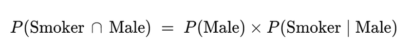
The full formula instead looks like that:

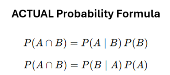
Now this formula gives us the consistency we need. To compute the probability of a male smoker, we substitute in the values like this:

Now, the final computed probability is identical to our tree diagram — and we resolved the mystery of why the probabilities did not seem to align previously.

Why Are There 2 Versions of the Intersect Formula?

If you are wondering about this — good for you! You are exhibiting excellent critical thinking. Indeed, the fact that there are two ways to compute the same term is key to Bayesian Statistics — but for now let’s focus on building the intuition for why the same term is represented in 2 different ways first. Honestly, the answer is simple. Consider these 2 tree diagrams:

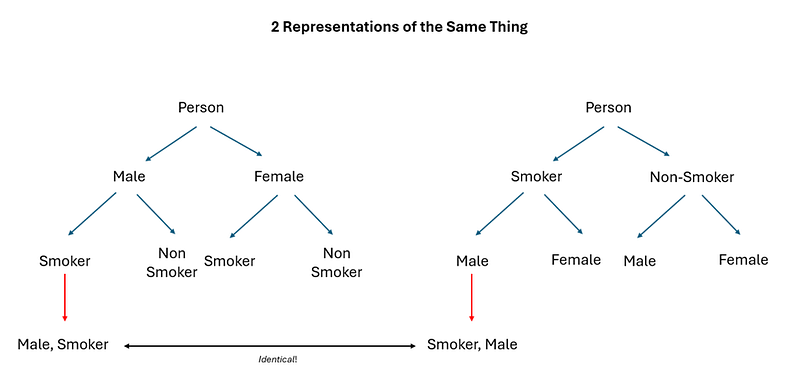
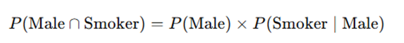
If you placed Gender as the first variable in the tree diagram (on the left), the formula you used to compute the probability of a Male Smoker would be:

If you placed Smoking Status as the first variable in the tree diagram (on the right), the formula you used to compute the probability of a smoker being male would be:

Obviously, the probability of a smoker being male, and the probability of a male being a smoker, are just different ways of phrasing the same term — male AND smoker. (This is a combination, not a permutation!) Which explains why the same probability can be written in 2 different formats — depending on which variable you put “first” in the tree diagram!

Venn Diagrams — Not Very Good for Showing Independence

When learning probability, we also commonly come across Venn Diagrams. We can depict the above gender x smoking scenario into a venn diagram as follows:

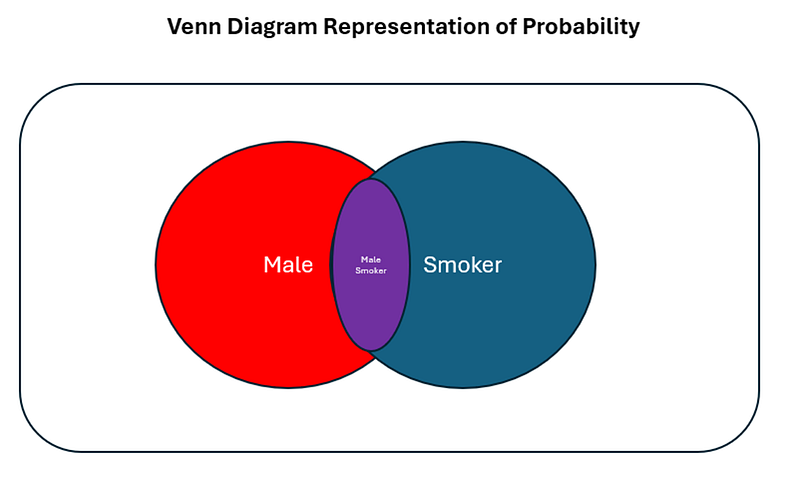
Now. My question to you is simple: from the above Venn Diagram, are gender or smoking status independent?

Think about this for a moment…

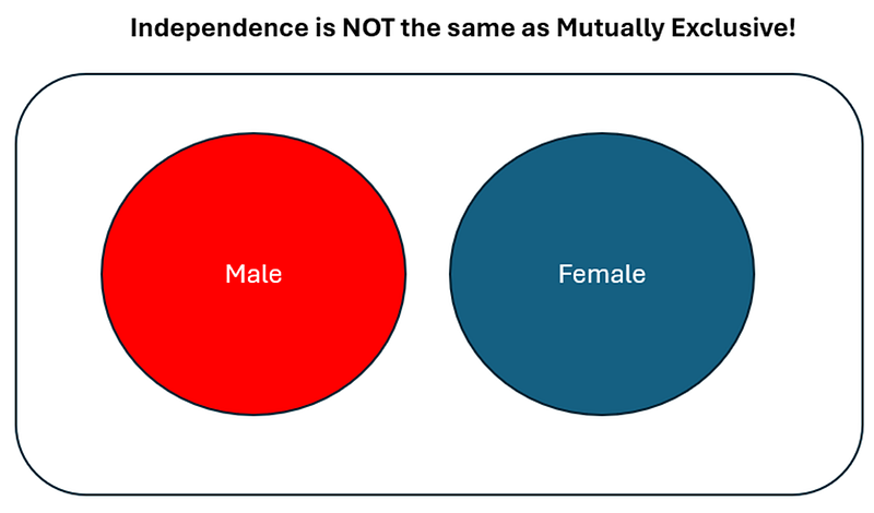
If you gave me a definite yes/no answer — congrats! You’re wrong. The correct answer is that you can’t tell independence from a Venn Diagram alone (can be both independent AND dependent). Some people mistakenly believe that independence = non-intersecting venn diagrams — this is NOT TRUE. Not intersecting = mutually exclusive (cannot both occur at the same time, e.g. cannot be male and female at the same time). This is not the same as independence — defined as knowing one variable not providing any information about the other variable!

Not understanding Venn Diagrams well is another reason why people get stuck when trying to learn Bayesian Statistics — their mental picture is wrong.

Don’t believe me? Let me drill it in further.

Venn Diagrams, Conditional Probability, and Independence

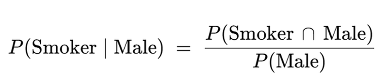
The conditional probability of being a smoker if you are male is given as follows:

Graphically, this corresponds to the purple area / red area in the venn diagram.

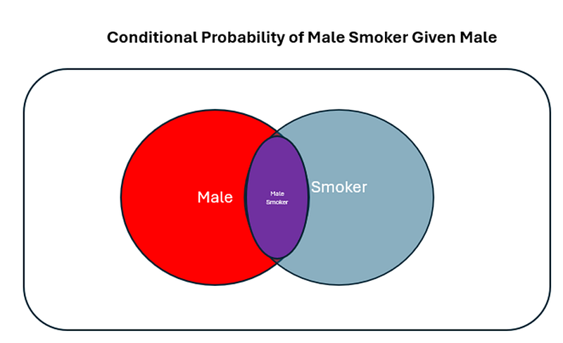
When we look at the computing the probability of a person being both male & a smoker, the formula is as follows:

Visually, this corresponds to the red area (male) multiplied by the purple/red area (smoker given male).

Substituting in our empirical numbers, the purple area is 0.42 (given by 0.5 x 0.8333). This is obviously not the same as 0.666 under independence — so the question is — how would the venn diagram look like under independence?

Independence as a special case of Dependence

Under Independence — the probability of being a male smoker is simply:

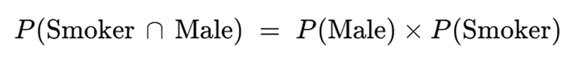
The the reason why this formula appears is simply because P (smoker) = P(smoker | male) under independence — because being male provides no information about whether or not you are a smoker (this is what independence implies!), these terms are equivalent.

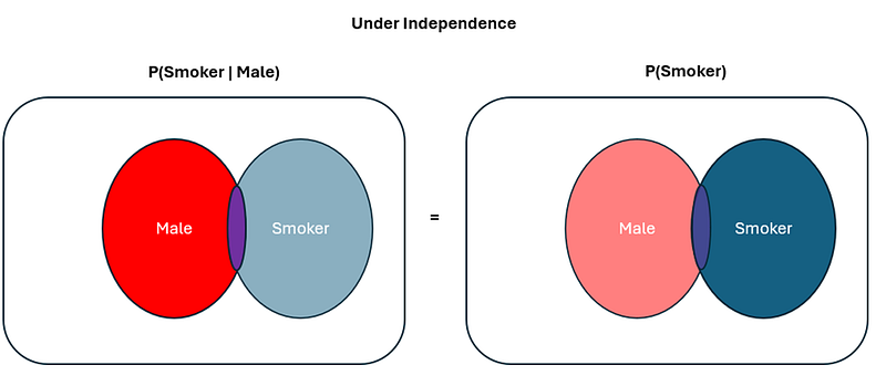
The question then is — how does P (smoker) = P(smoker | male) look in the Venn Diagram? P(smoker) is denoted by the blue area, whereas P(smoker | male) is denoted by the purple/red area. How are these 2 equivalent?

The Truth About Independence via Venn Diagrams

Simple fact — they’re not. Under independence, it is just so coincidental that numerically — P (Smoker | Male) = P(smoker). In truth, even under independence, these probabilities are referring to completely different things — one has the males as the denominator (P(smoker|male), whereas the other has the entire sample space as the denominator (P(smoker)). It just so happens that numerically, under independence, these two probabilities are numerically the same — even though in actuality, the areas in which they represent in the Venn Diagrams are fundamentally different. This was what trips people up most of the time — because intuitively we think that if numerically the probabilities are the same, they must refer to the same area in the Venn Diagram — not knowing numerical equivalent does not literally equate to space equivalence in the context of Venn Diagrams.

In truth, via venn diagrams, you CANNOT tell whether something 2 events are independent unless specifically given the probabilities of the intersection and testing if it is equivalent to P(A) x P(B). Put graphically:

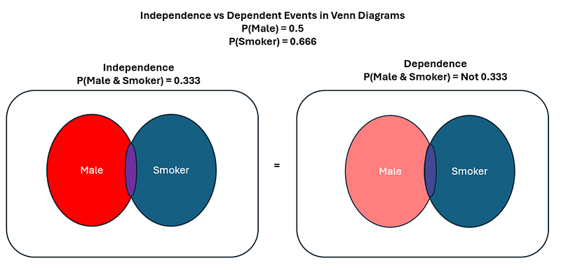
Notice how in both dependence & independence, visually the Venn Diagram looks exactly the same. The only way you can tell whether the events are independent is via computing the probability of the intersection, and seeing if numerically, it corresponds to P(Male) x P(Smoker) which is 0.333 in this context. If it is, then events are independent. If it is not, then the events are NOT independence. With our empirical numbers, we know that the purple area was computed to be 0.42 — which is not 0.333. As a result, in our scenario, the gender & smoking status are NOT independent. (equivalent to rejecting the null hypothesis).

Conclusion

Wow! That was long! In this post, we transition from frequentist to bayesian probability, understanding why people often fail to properly understand Bayesian statistics. Indeed, the main hurdle comes from “independence” being the default state of modelling — in frequentist perspective, we only set the null hypothesis (independence), the try to disprove it. Which is why we are so unfamiliar with conditional probabilities.

The problem is made worse as when we try to use Venn Diagrams to understand conditional probabilities, we often just stuck because we fail to realise that Independence can’t really be “seen” inside this tool of choice. As a result, we just proceed on with this niggling feeling that something is wrong, yet are unable to fully pinpoint what exactly.

I hope this post gave you the tools you need to probability understand conditional probability, and stay tuned for more as I breakdown Bayesian Statistics in detail!